Preprint 2026 · Daedalus

Self-Supervised Learning of Universal Latent Spaces for Operator Learning

Sepehr Mousavi1,3,  Levi Lingsch2,3,  Siddhartha Mishra2,3,  Laura De Lorenzis1,3
1Department of Mechanical and Process Engineering, ETH Zurich   2Seminar for Applied Mathematics, ETH Zurich   3ETH AI Center
ETH Zurich Computational Mechanics Group CAMLab ETH AI Center

TL;DR  We pre-train one autoencoder on synthetic functions only, freeze it, and reuse its latent space for every operator. It reconstructs PDE solutions and photographs on geometries it never saw, its latent space is interpretable, and operators trained on cached embeddings match or beat end-to-end models at a fraction of the cost.

a field, its partitions, and two of them at their own scale
scroll
23/28
problems where the frozen-latent operator beats the strongest end-to-end baseline (GAOT); all 24 against RIGNO
2.1×
faster training than the best baseline on average, 8.3× faster than RIGNO
1.4 GB
training memory of the latent mode (batch 32), unchanged from 4,096 to about 67 million points per function
0
PDE solutions seen in pre-training: the backbone learns from analytic functions synthesized on the fly
The method

From one function to a latent operator

One autoencoder, trained without labels, turns any function on any point cloud into embeddings on a hypersphere and back. The four steps below run on the real model, the first three on the paper's 8-dimensional backbone so that every embedding can be shown in full; click a step to jump to it.

Read the method in detail →

Interactive · pre-computed

Do latent geodesics follow the physics?

An incompressible flow (IEU-BB, velocity u) evolves over 20 steps. Every K-th snapshot is an anchor; every state in between is decoded from the great circle (SLERP) between the two nearest anchor embeddings, without any operator. On the globe, the physical evolution traces a curve, and the geodesics cut across it.

Latent hypersphere illustrative projection

physical evolution geodesic between anchors snapshot active anchors drag to turn

Physical evolution t = 0

ground truth

Geodesic estimate

anchor

Error of the geodesic estimate relative L2

geodesic vs. truthreconstruction flooranchors
Right now
0%
geodesic error
0%
autoencoder floor

Between anchors close in time, the geodesic stays within a few percent of the true flow: the embedding preserves the geometry of the evolution. Spread the anchors (K = 10) and the shortcut drifts off the physical path: over longer intervals, following the physical path is the job of a learned operator.

Interpretability

Directions in the latent space mean something

The chord between the embeddings of two anchor fields that differ by one operation is a direction. Added to the embedding of a different field, it applies the same operation. Scroll over the field or drag the slider.

Direction
anchor A
anchor A ·
→
anchor B
anchor B ·

Field it is applied to
c = 0

z → |z| (z + c d) / |z + c d|, decoded with the identity frame on a square grid, each strip on its own colour scale, so only the shape changes. Apply it to your own field →

Findings

What a frozen, universal latent space buys

∞

Universal by construction

Partitions and their normalization carry a field into the familiar band of the training functions, provided it is sampled finely enough to be partitioned, so one backbone serves fluids, solids, waves and images on unseen geometries.

↻

Exactly equivariant

The representation is exactly equivariant to translation, dilation and amplitude: the static frame stores them, the embedding carries only the shape.

✦

Interpretable

The whole latent space is used and decodes to valid fields, latent distances preserve the order of distances between the decoded fields, geodesics interpolate evolutions, and edit directions transfer. More →

⚡

Fast and lean operators

A dataset is encoded once and an operator trains on cached embeddings. Latent rollouts run up to 10× faster than re-encoding at every step (up to 9.6× faster than the best baseline on variable point clouds), and a 101M-parameter processor trains on 262k-point functions on one consumer GPU. More →

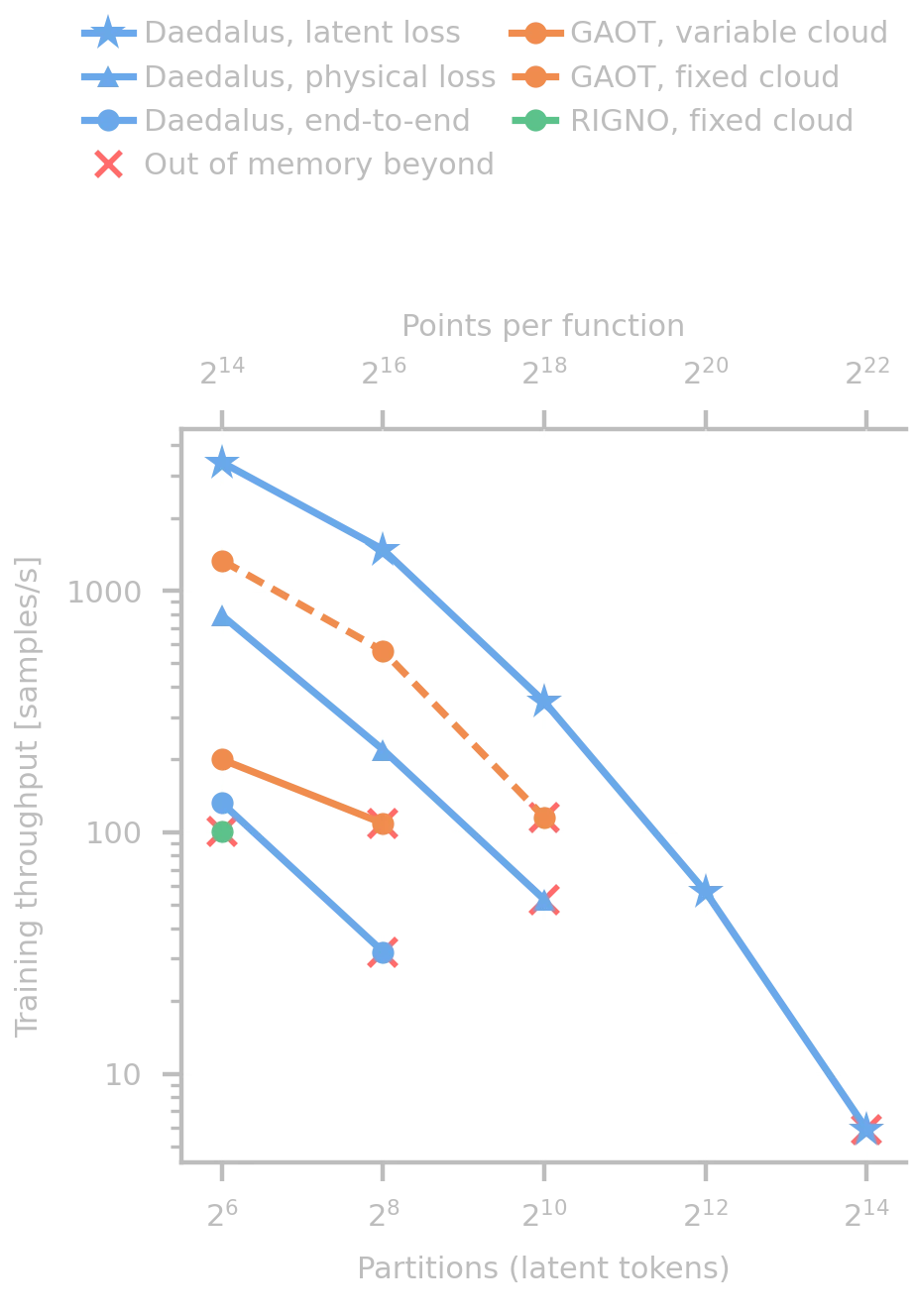
Training throughput against the number of partitions on log axes: the latent-loss training of Daedalus stays fastest and reaches 16384 partitions, while the other settings run out of memory far earlier
Training throughput on one 24 GB RTX 4090 as the partitions grow, at 256 points per partition and a batch of 32. Daedalus trains on the latent loss with input and output caches (stars), on the physical loss with an input cache (triangles) or end to end (circles); GAOT trains end to end on a cloud per sample (solid) or one cloud per batch (dashed), RIGNO on one cloud per batch. A red cross marks where a line runs out of memory. All benchmarks →
Bars of the mean relative L1 test error and the mean training time of Daedalus, GAOT and RIGNO-12 for every family of the 28-problem benchmark and over all problems; Daedalus has the lowest error everywhere and the shortest training time on most families
Mean relative L1 test error and training time of the operator on the frozen backbone and of two end-to-end baselines, per family of the 28-problem benchmark (problems per family in parentheses) and over all problems. A bar that reaches the end of an axis is cut there. RIGNO-12 is not trained on the steady compressible flows, so its overall mean covers 24 problems. Per problem →
Live demos

Run the backbone on your own input

Eight demos run the frozen 128-dimensional analysis backbone on a small CPU server. Every demo comes with pre-computed samples that show at once; your own inputs are queued and run one at a time.

Cite

BibTeX

@article{mousavi2026daedalus,
  title   = {Self-Supervised Learning of Universal Latent Spaces for Operator Learning},
  author  = {Mousavi, Sepehr and Lingsch, Levi and Mishra, Siddhartha and De Lorenzis, Laura},
  journal = {arXiv preprint (placeholder)},
  year    = {2026}
}